This is my attempt to turn an interesting paper I’ve read into some notes. I will introduce a recently published article and share my findings from trying to replicate it.
Reference: Y. Wang, M. Wei, Z. Ye, T. Hu, and H. Zheng, “An adaptive tone mapping method for PQ ‐ and HLG ‐encoded HDR contents,” Color Res. Appl., p. col.70002, July 2025, doi: 10.1002/col.70002.
This is an adaptive tone mapping algorithm that maps 0-1000 nits HDR content to 0-100 nits SDR. It consists of three parts: tone compression, detail enhancement, and dark area enhancement.
A Special Kind of Luminance
The concept of Luminance in this algorithm is quite special. It is not the Y from the XYZ colour space, but rather the maximum of the RGB values, similar to the Value in HSV.
This definition of luminance is used to ensure that values always stay within the RGB space during compression, preventing drastic hue shifts that could be caused by going out of gamut. However, it is worth noting that even if the chromaticity coordinates remain the same, a change in luminance can still alter perceived hue and chroma. An example of this is the Bezold–Brücke phenomenon, which describes how our perception of hue can change with light intensity.
Throughout the paper, ’luminance’ refers to this specific concept. The RGB space is always linear Rec. 2020. This article does not cover gamut compression; the output is an image in the Rec. 2020 space but with an SDR luminance range.
The Tone Compression Curve
The tone compression curve is applied to the special luminance mentioned earlier, compressing the range from 0-1000 down to 0-100. This curve is formed by a linear segment and a rational function, creating an overall shape that resembles a roll off. The entire curve lies below the y=x line, which means no part of the image is brightened in this step.
The curve is designed around a few specific luminance points, with the function’s coefficients calculated to connect them smoothly.
In Appendix 4.2 of the ITU-R BT.2408 report, it is noted that skin tones on an HLG display with a peak luminance of 1000 nits should correspond to 45% to 56% of the HLG signal (with an average of 50%). On an SDR display with a peak luminance of 100 nits, they should correspond to 61% to 82% of the SDR signal (with an average of 70%). Therefore, the luminance of skin tones is approximately 50.7 nits in HDR content and 42.5 nits in SDR content. This 50.7 nits value is also used as the knee point between the linear segment and the curve.
Another pair of luminance points is for diffuse white. In a 1000-nit HDR system, the recommended luminance for diffuse white is 203 nits. In an SDR system, it is typically set to a 92% signal value, which is about 81.7 nits.
Detail Decomposition and Enhancement
Compressing luminance leads to a loss of detail, especially in the highlights where textures become hard to distinguish due to reduced contrast. Before compressing the luminance, a bilateral filter is used to separate the base layer from the detail layer. Tone compression is applied only to the base layer. The detail layer, on the other hand, undergoes an additional enhancement process to suppress potential halos around high contrast edges in the image.
The paper provides a set of recommended empirical values for the three main parameters of the bilateral filter: window size, spatial variance, and range variance.
The additional detail enhancement is based on the local variance of the area surrounding a pixel and the global variance of the entire image. However, the relevant formulae in the paper are almost all incorrect and the textual descriptions are brief, so I have not yet been able to fully replicate this part.
$$ \sigma_G = \sqrt{\frac{\sum_{p \in I} \left( L_{\mathrm{HDR}}(p) - \overline{L}_{\mathrm{HDR},I} \right)}{N}} $$$$ \sigma_L(p) = \sqrt{\frac{\sum_{q_i \in \Omega_i} \left( L_{\mathrm{HDR}}(q_i) - \overline{L}_{\mathrm{HDR},\Omega_i} \right)}{N_i}} $$The two formulae above are from the paper, but their results are always 0. If you add squares to make them variance or standard deviation calculations, the subsequent steps still do not work correctly.
Broadly speaking, the idea is to first calculate the variance (or possibly standard deviation) of all pixels in the entire image. Then, for each pixel, you calculate the variance or standard deviation of the surrounding neighbourhood. A threshold is set based on the global variance, and only the details corresponding to areas exceeding this threshold are enhanced.
Dark Region Enhancement
After the first two steps, we have an image suitable for an SDR display. Most images do not need this final step. In my tests, the dark area enhancement is only triggered when the average luminance of the input image is below about 1 nit. The clustering I implemented with SciPy is very slow, but the brightening effect from this step is quite good.
Since the tone compression curve is always below the y=x line, it reduces the image’s overall luminance. If the original content is already quite dark, the output image might become too dim, a problem exacerbated by the poor performance of SDR transfer functions in dark regions. The authors therefore designed an optional module to enhance dark areas. This module is activated only if the average luminance of the mapped image is below a certain threshold; otherwise, the image is output directly.
First, all pixels in the image are grouped into 64 clusters based on their luminance. The average luminance of each cluster is calculated and stored in a 64 element vector. Two gamma values are set, for instance, 1 (for the brightest cluster) and 2.2 (for the darkest cluster). The other 62 gamma values are derived through linear interpolation, with the intervals determined by the average luminance of the clusters.
Then, the reciprocal of these gamma values is applied to the luminance of the pixels in each respective cluster, brightening the image. This acts as a dynamically adaptive system gamma.
Results
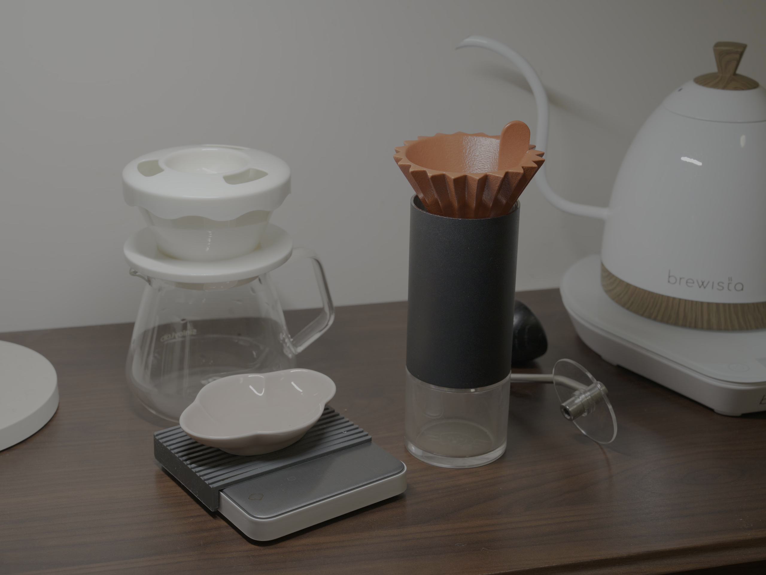
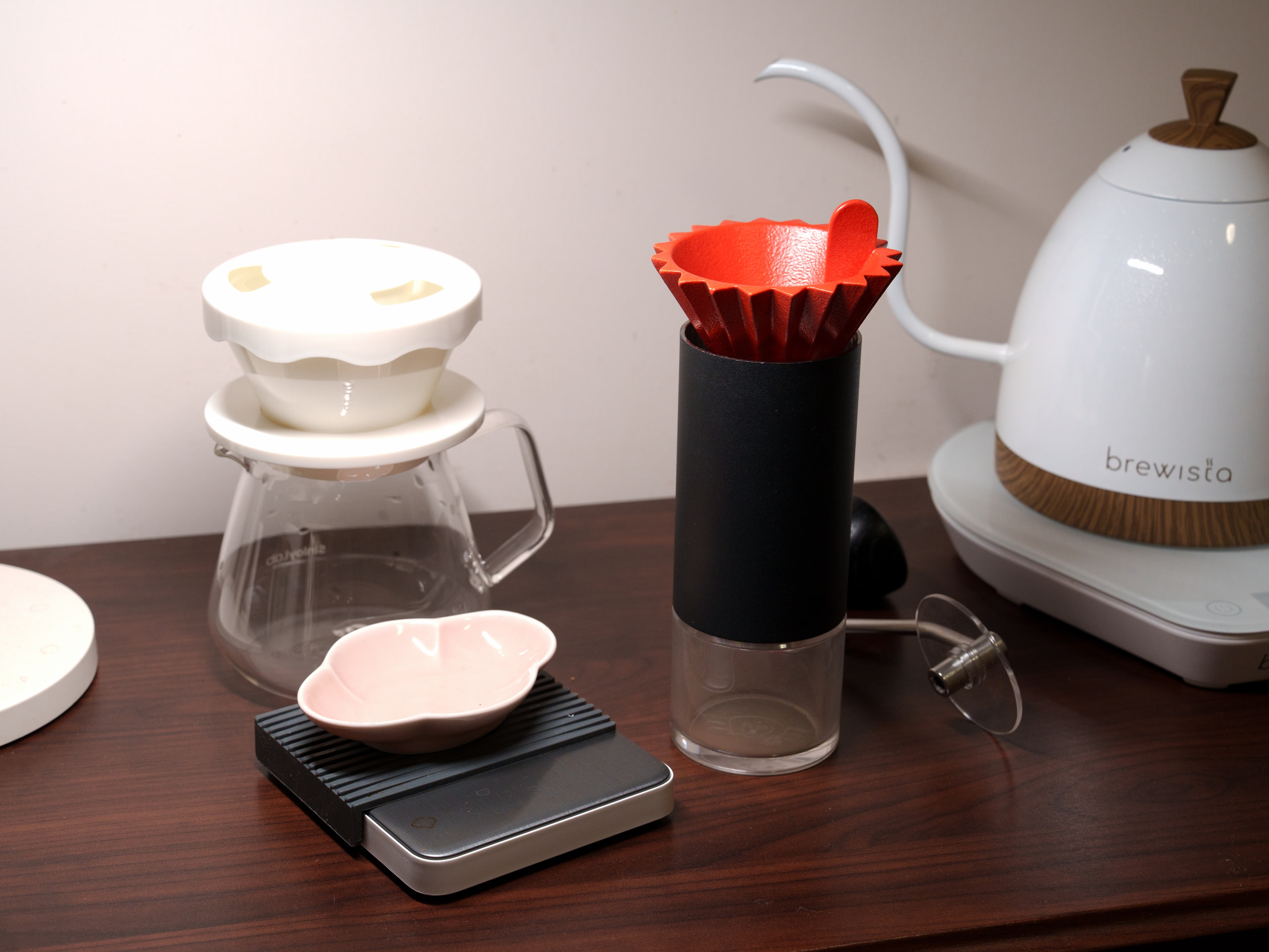
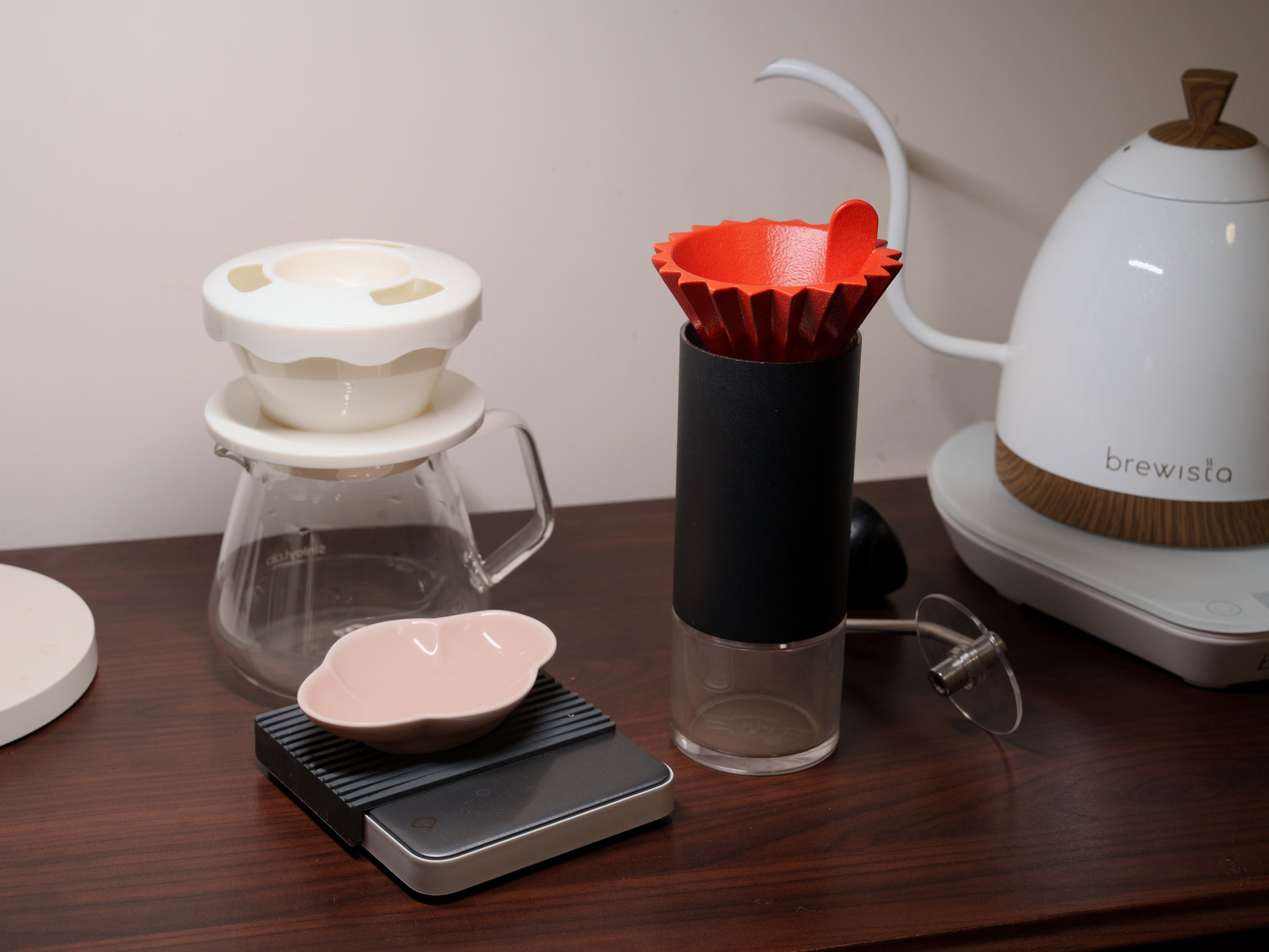
I tested the algorithm using a post processed photo. During editing, I controlled the luminance of different elements in the image to adhere as closely as possible to HDR production standards. If your display is not capable of showing the full HDR luminance range of the image, Chrome should perform Tone Mapping. Apart from the first image, all subsequent images are SDR.

If we simply clip any values above the nominal SDR luminance, parts of the image become pure white.

With the partially replicated detail enhancement turned off, which means only applying the tone compression curve, the highlights in the image are recovered quite well.

By modifying the detail enhancement formula to calculate standard deviation and using a manually specified threshold, I got a more complete result. You can see some processing along the high contrast edges.

Although I couldn’t fully replicate the detail enhancement, the tone compression curve applied to the special luminance already produces good results and is very fast. In contrast, the bilateral filter and local variance calculations needed for detail enhancement are computationally expensive.
It must be pointed out, however, that the core of this algorithm is the tone compression curve, which is designed based on HDR and SDR production standards and experience. If the HDR content was not created according to these standards and has a more “freestyle” luminance distribution, the results may not be as effective.
Once all the details and potential errors in the algorithm are confirmed, I will refine the article. It would be ideal if the code could be made open source.
