Schrödinger’s Optimal Pigments
Yes, that Schrödinger.
As early as 1920, Schrödinger published a paper titled Theorie der Pigmente von größter Leuchtkraft. The original text was in German, but thankfully, we now have multilingual LLMs to help. The paper broadly discusses the reflective properties of various pigments, why the colour saturation achievable by pigments is less than that of pure spectral light, and deduces a theoretical “optimal pigment”. This pigment has a binary reflectance spectrum with respect to wavelength—it either reflects light completely or not at all.
At that time, the CIE had not yet introduced the CIE 1931 XYZ colour matching functions, and this was also before the 1924 $V(\lambda)$ function. The definition of “luminance” (Helligkeit) in the paper was related to a “quantity” (Quantität), which was a combination of three colour quantities—a precursor to later concepts of colour matching functions and luminance. Discussions about optimal colours began even when fundamental concepts like luminance were still vague, making it one of the topics with the richest history in colour science.
MacAdam’s Optimal Colours
By 1935, with quantified standards for luminance and colour established, MacAdam published a paper proposing the concept of optimal colours, described in the original text as “Maximum Visual Efficiency of Colored Materials”.
MacAdam’s optimal colours form the outer surface of the “theoretical object colour solid” in the luminance dimension. That is, they represent the upper limit of luminance for the set of colours that any object relying solely on reflection (non-fluorescent, non-emissive) can theoretically produce under a specific illuminant. This solid is defined by all physically possible reflectance spectra and contains all real object colours, with its surface representing the theoretical limits.
An Optimal Colour refers to the colour corresponding to the maximum achievable luminance for each set of chromaticity coordinates (x, y or u’, v’), i.e., “the theoretical object colour with the highest luminance for a given chromaticity”. For example, here is a false-colour plot of the luminance of MacAdam’s optimal colours under a certain illuminant.
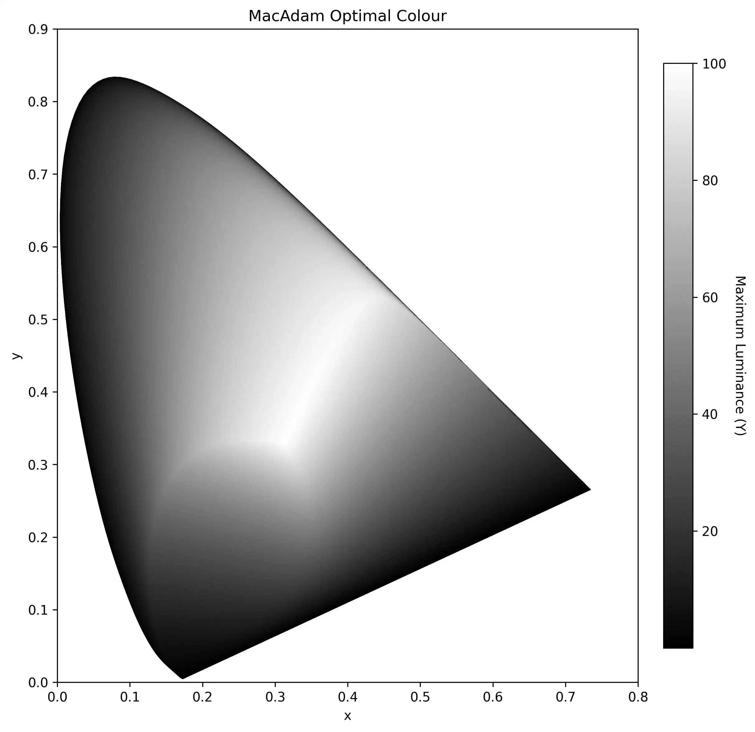
The reflectance functions required to achieve these optimal colours take the form of a “binary square-wave” with only two transition points. Although such reflectance spectra are impossible to achieve in reality, they constitute the theoretical ceiling for object colours.
Proof of the Square-Wave Reflectance
Both Schrödinger and MacAdam proved that to achieve an optimal colour, its reflectance must be a binary square-wave with no more than two transition points. Their proofs were based on physical analysis and intuition.
Below, we will use the calculus of variations and the Lagrange multiplier method to prove mathematically that for any given chromaticity coordinates, the reflectance that achieves maximum luminance is a “square-wave”.
Let’s first express these conditions and the problem in mathematical language:
The Problem Statement
- Reflectance R, a function of wavelength $\lambda$, with values between 0 and 1.
- Colour Matching Functions (CMFs), used to convert a spectral power distribution into tristimulus values XYZ, are also functions of wavelength, denoted as $\bar{x}$, $\bar{y}$, and $\bar{z}$.
- The spectral power distribution of the illuminant I and the reflected spectral power distribution P.
- Any given chromaticity coordinates $x_0$, $y_0$.
To prove: for given chromaticity coordinates $(x_{0}, y_{0})$, there exists a reflectance function $R(\lambda)$ that maximises $Y$. At this maximum, the value of $R(\lambda)$ can only be 0 or 1.
Detailed Proof
We can prove using the calculus of variations and the Lagrange multiplier method that for any given chromaticity, the reflectance spectrum that achieves maximum luminance must be a “square-wave” function, taking values of only 0 or 1.
To make the derivation clearer, we will proceed in two steps: first, proving the conclusion under an idealised equal-energy illuminant; then, generalising this conclusion to any illuminant to show that the illuminant’s spectral distribution does not affect the “square-wave” form of the optimal reflectance.
Step 1: Proof under an Equal-Energy Illuminant
Let’s first assume the illuminant has an equal-energy spectrum, meaning its spectral power distribution $I(\lambda)$ is a constant. To simplify calculations, we can set $I(\lambda)=1$ and $k=1$. The tristimulus values are then:
$$ X = \int R(\lambda) \bar{x}(\lambda) \, d\lambda, \quad Y = \int R(\lambda) \bar{y}(\lambda) \, d\lambda, \quad Z = \int R(\lambda) \bar{z}(\lambda) \, d\lambda $$Our goal is to maximise luminance $Y$ subject to the chromaticity coordinate constraints $(x_0, y_0)$. The objective function is:
$$ \text{Maximise} \quad Y = \int R(\lambda) \bar{y}(\lambda) \, d\lambda $$The chromaticity constraints $x=x_0$ and $y=y_0$ can be transformed into two equivalent linear constraints. For notational simplicity, we define $z_0 = 1 - x_0 - y_0$. The constraints are:
$$ \int R(\lambda) \left( \bar{x}(\lambda) - \frac{x_0}{y_0} \bar{y}(\lambda) \right) d\lambda = 0 $$$$ \int R(\lambda) \left( \bar{z}(\lambda) - \frac{z_0}{y_0} \bar{y}(\lambda) \right) d\lambda = 0 $$This is a constrained optimisation problem. We introduce Lagrange multipliers $\mu_1, \mu_2$ to construct an auxiliary functional $J[R]$. By combining the objective function and the constraints, the problem is transformed into maximising $J[R]$:
$$ J[R] = \int R(\lambda) f(\lambda) \, d\lambda $$where the core part of the integrand, $f(\lambda)$, is given by:
$$ f(\lambda) = \bar{y}(\lambda) - \mu_1 \left( \bar{x}(\lambda) - \frac{x_0}{y_0} \bar{y}(\lambda) \right) - \mu_2 \left( \bar{z}(\lambda) - \frac{z_0}{y_0} \bar{y}(\lambda) \right) $$Rearranging the above equation by the colour matching functions (CMFs), we get:
$$ f(\lambda) = c_1 \bar{x}(\lambda) + c_2 \bar{y}(\lambda) + c_3 \bar{z}(\lambda) $$Here, $c_1, c_2, c_3$ are constants that depend only on $(x_0, y_0)$ and the multipliers $(\mu_1, \mu_2)$. This shows that $f(\lambda)$ is always a linear combination of the CMFs.
To maximise the integral $J[R]$ under the physical constraint $0 \le R(\lambda) \le 1$, we must independently maximise the integrand term $R(\lambda) f(\lambda)$ at each wavelength $\lambda$:
- If $f(\lambda) > 0$, we should choose $R(\lambda) = 1$.
- If $f(\lambda) < 0$, we should choose $R(\lambda) = 0$.
- If $f(\lambda) = 0$, the value of $R(\lambda)$ does not affect the result, and these points form the transition points from 0 to 1.
Therefore, the optimal reflectance $R(\lambda)$ can only take values of 0 or 1. Its graph has a “square-wave” shape, and its transition points are the zero-crossing points of this linear combination of CMFs.
Step 2: Generalisation to Any Illuminant
Now, let’s consider an arbitrary illuminant $I(\lambda)$, where $I(\lambda) > 0$. The tristimulus value formulae become:
$$ X = k \int R(\lambda) I(\lambda) \bar{x}(\lambda) \, d\lambda $$and similar forms for $Y$ and $Z$.
Repeating the derivation above, each integral term in the objective function and constraints will be multiplied by $I(\lambda)$. The final auxiliary functional becomes:
$$ J[R] = \int R(\lambda) I(\lambda) f(\lambda) \, d\lambda $$where the definition of $f(\lambda)$ is identical to that in the first step. It is still a linear combination of the CMFs, and its form does not depend on the illuminant.
To maximise $J[R]$, we need to maximise $R(\lambda) I(\lambda) f(\lambda)$ at each wavelength. Since the illuminant’s spectral distribution $I(\lambda)$ is always positive, the sign of this term is determined entirely by the sign of $f(\lambda)$. Therefore, the strategy for choosing $R(\lambda)$ is exactly the same as in the first step.
This proves that for any illuminant, the optimal colour at a specific chromaticity must correspond to a square-wave reflectance spectrum with values of only 0 and 1. Its “shape” (i.e., the positions of the 0/1 transition points) is determined solely by the linear combination of the CMFs and is independent of the illuminant.
Calculation Method for MacAdam’s Optimal Colours
One direct approach is: for a given set of chromaticity coordinates xy, solve for the corresponding Lagrange multipliers $\mu_1, \mu_2$, then find the zero-crossing wavelengths of the linear combination of CMFs, and use these to construct the square-wave reflectance and calculate the corresponding luminance. However, solving for the Lagrange multipliers from xy is a non-linear process with no explicit solution. Instead, the problem can be approached from another angle to quickly solve for the optimal colour’s luminance.
The key insight is that a linear combination of the CMFs can, in most cases, produce at most two zero-crossing points (excluding the endpoints), making the square-wave reflectance either a band-pass or a band-stop filter.
Using this property, we can quickly iterate through all possible reflectances to build a two-dimensional look-up table that returns the maximum luminance for a given set of chromaticity coordinates.
The specific procedure is to define two cut-off wavelengths, $\lambda_1$ and $\lambda_2$. One moves from short to long wavelengths, while the other moves from long to short wavelengths. For each pair, we calculate the chromaticity coordinates and luminance for both the band-pass and band-stop reflectances they define. This generates a look-up table of the form $Y=f(x,y)$.
Significance
MacAdam’s optimal colours serve as a theoretical benchmark for measuring the colour reproduction capabilities of devices like printers. The gamut of any reflective device cannot exceed the boundaries defined by the MacAdam limits, providing a theoretical ceiling for the development of colour management and wide-gamut technologies.
In the age of HDR, the concept of MacAdam’s optimal colours seems poised to find new applications and offer fresh inspiration.